Volume & mix
Tonnage by grade family, dimension band and plant. Agreed in S&OP, and then held to — with variance tracked rather than quietly forgotten.
Demand planning, multi-plant capacity planning and production planning built on the same material and route model the schedulers use — so the plan and the schedule are never arguing about different data.
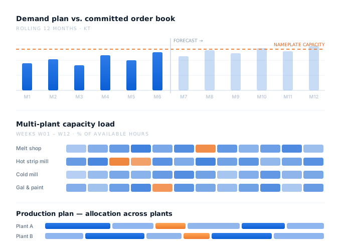
Forecast, firm order intake and contract call-offs on a single horizon — with the netting rules that stop a contract being counted twice.
Metals demand is rarely a clean forecast. It is a mix of annual contracts with monthly call-offs, spot business that arrives late and demands early, and a sales team with a view about next quarter. The planning layer has to hold all three without double-counting, and has to be honest about which part of the number is actually committed.
Committed versus forecast, split by contract and spot.
By grade family and by plant, before sales promises it.
So the conversation happens in month two, not month eleven.
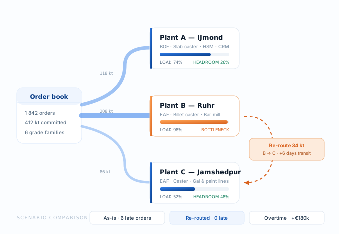
Most metals groups run several plants that quietly compete for the same order book. Allocation usually happens in a spreadsheet owned by one person. We make it explicit.
Two plants can both make a grade, but not at the same cost, not on the same lead time and not with the same yield. Capacity planning has to weigh all three, plus transit, plus what is already loaded — and then show its work, because someone will challenge the answer.
The layer that turns an allocated plan into something a scheduler can actually execute — monthly, then weekly, then handed over cleanly.
Tonnage by grade family, dimension band and plant. Agreed in S&OP, and then held to — with variance tracked rather than quietly forgotten.
Group the month into campaigns the units can actually run: cast sequences, rolling programmes, coating blocks, colour runs.
Released as a constrained work list, not a wish. The scheduler sequences inside it and reports back when it cannot.
A planning tool that does not know what is physically in the yard will keep planning production you do not need. Because our planning layer sits on the same material model as DigiPlantMES, available stock, work in progress and actual yields feed the plan continuously.
That closes the loop most implementations leave open: the plan learns that a route yields 91% and not the 94% in the master data, and next month's plan is right for the first time.
Actual route yields replace master-data assumptions, per grade and per unit.
Planned production nets against what is already made and sitting in the yard.
Available-to-promise that reflects real route capacity rather than an offset in days.
Plans are wrong the moment a caster trips. What matters is how quickly you can build a defensible alternative and see what it costs.
Take a unit down for four days and see the whole horizon re-flow, with the orders that become late listed by customer.
Test a large enquiry against real capacity before sales commits a date to it.
Move volume between plants and see cost, transit and lead-time consequences side by side.
Longer campaigns for efficiency versus shorter ones for service — priced, not argued.
Every scenario keeps its assumptions. When someone asks in November why the October decision was made, the answer is a record rather than a recollection.
Planning and execution are one product with two entry points. Some customers start with multi-plant allocation; others start with tracking on a single line. Both work.